Excell Skip Hit Chart

Frank

Member
This is my attempt at getting instantaneous skip readout for 649 without bonus. Assumes the data starts with draw 1 at the top down to the most recent draw at the bottom and all draws are numbered.

https://www.mediafire.com/?oekkcqt503ajta2


As I mentioned earlier, I don't think the original LOOKUP formula format can scan multiple columns, so if you are looking for the latest ocurrence of a ball which might appear in any of 6 columns, you need 6 versions of the formula checking six columns. I dispensed with the ABS part of the formula, it was superfluous in this case.

It is not necessary to instantly calculate a skip because that depends on which of the six columns holds the most recent ocurrence and its draw number. Initally that part of the calculation is left out of the formula, we just need to find the most recent draw number for each number per column.
So for 49 balls drawn in six columns thats 49 x 6 calculations followed by 49 more calculations to assess the most recent draw number per ball, hence the skip.
I created a grid of calculating cells along seven rows to accomplish this. However, how does one know where to start looking up from when users can add new draws to the bottom of the list? I had to use the OFFSET function to find the row number of the last draw in the table, helped by a draw counter in a named cell - called Maxdraw. So the original LOOKUP idea was modified to use the column headers (in particular Cell B12) as a datum to work from to find the last result.

I ended up with a 49 x 6 row counting grid containing the draw numbers of each number's last ocurrence. However not every number appears in every column, and where they don't, I was getting N/A in those cells. So I had to check each cell for the N/A message and replace each with a "" (blank), making the formula even more complicated.
By finding the Max of the six rows per number, I got the last appearance draw number. Then the final 49 formulas subtracted these from the current draw number to get the skip.

Assumptions:- a 649 lottery bonus ball not included.

most recent draw number at the bottom

draws numbered ascending downwards.
 

Frank

Member
Thank you Bloubul, that version expects data to be in ascending order because the grey cells at the ends of the table have no formulas in them. It could be modified easily to allow data in any order by copying the existing formulas along to the ends of the rows. Its easy to remove the protection, there is no password needed.Remove it at your own risk. :rolling:


My preferred way of working is to actually have the latest draw at the top, and the oldest draw at the bottom, which creates different challenges in writing formulas. Once one has overcome the problem of inserting a new row to hold the latest draw, (done by a macro in my version), the easiest way to check for the latest ocurrence looking downwards could be the VLOOKUP command, however it only works when the draw number is to the right of the results. Ideally they are to the left of the results.

The replacement formula which allows looking to the left of ball numbers to read off draw numbers is a combination of the INDEX and MATCH functions, which nested together do the trick.
The other problem to get around is that everything scrolls down when you insert a new line, but you need the checking formulas to stay rooted to the top of the results and not move down with them. Thats why the OFFSET function is in the formulas, working from the header row which always stays fixed at row 12. To blank out N/A messages, I again had to add the ISERROR function to filter them out and show a blank.

This version then is different in three ways from the above,

1. It has a macro to insert new draws
2. It can have results in drawn order and still work
3. Your data set needs the latest draw to be at the top.

https://www.mediafire.com/?r3mmlux4o3xcggx

I think this excercise proves that there can be no SIMPLE single formula that can display current skips for lotteries ! :)
 

Frank

Member
bloubul said:
cdrake..

Where can I download the Irish Lotto in drawn order from day 1 please.

BlouBul :cool:

cDrake has been back and not responded.

The problem with the Irish Lotto is that it's changed its matrix about three times since the 1980's. It's been 6/36, then it was 6/42, then it was 6/45, and since September this year it's been 6/47. What's the point of knowing the results since the 1980's? How will it help?

Since Saturday 5th September it's been 6/47, and there's the main lotto, plus 1 and plus 2. You need to be clear which of these you need.

http://www.irishlottery.com/archive.asp

This will give you main lotto results, but it's not a CSV file, it's hard labour typing in the results. However, in my opinion you only need to go back to the last change of matrix in September.
 

Icewynd

Member
Bloubul,

I have e-mailed my lottery and had them send me results in .csv format. Maybe Irish lotto will do the same? There should be a contact e-mail listed on their website.

Good Luck!
:thumb:
 

Frank

Member
You can create a text file month my month, if you set the parameters. I suggest going back to September 9th 2015 when the 6/47 format started. Copy and paste from the web page to notepd.


http://www.lottostrategies.com/script/winning_select_state/272/IE/irish-lottery-numbers-archive.html

I did the last 3 months and converted to CSV:-

Day,Date,N1,N2,N3,N4,N5,N6,B
SAT,11/28/15,3,7,17,24,26,29,40
WED,11/25/15,2,5,7,16,46,47,15
SAT,11/21/15,3,9,13,27,38,44,14
WED,11/18/15,5,7,10,16,30,46,32
SAT,11/14/15,12,16,22,36,40,43,4
WED,11/11/2015,3,5,14,30,40,43,45
SAT,11/07/2015,5,8,9,10,15,29,17
WED,11/04/2015,1,5,8,19,20,28,3
SAT,10/31/15,3,8,15,25,39,45,28
WED,10/28/15,5,7,10,18,41,47,44
SAT,10/24/15,3,12,15,19,23,32,20
WED,10/21/15,10,11,36,41,44,46,45
SAT,10/17/15,4,7,19,22,25,41,8
WED,10/14/15,8,13,16,18,30,31,39
SAT,10/10/2015,1,21,34,36,38,40,5
WED,10/07/2015,8,12,13,28,34,46,44
SAT,10/03/2015,1,15,17,31,36,45,18
wED,09/30/15,4,9,27,31,38,39,10
SAT,09/26/15,4,8,26,28,34,38,30
WED,09/23/15,5,6,14,16,32,43,27
SAT,09/19/15,7,26,34,39,41,42,31
WED,09/16/15,3,9,22,25,27,31,23
SAT,09/12/2015,6,12,15,17,32,40,21
WED,09/09/2015,2,6,21,26,43,45,12
SAT,09/05/2015,7,9,17,20,26,27,40

Thats all the data since it changed.
 

Cartref45

Member
Hi,

This is my first attempt to upload a file via Mediafire, try this link and let me know if it s available - http://www.mediafire.com/view/k0r0zclh2c6rsl6/HitSkip-TB.xlsx

This is a spreadsheet that I use to analyse number skips for my Lottery - Thunderbal 5/39.

There are 2 sheets one which is updated every draw and the other updates the skips for each ball. To update just insert row and add new draw in the 1st sheet (NUMBERS), should be easy to adapt for any lottery.

I am only a novice with Excel and I am sure some of the seasoned Excel programmers could improve.

The 2nd sheet (Hit&Skip -MB) gives the skip for the last 20 skips of each ball and the "dueness" at the time it appeared, based on an average of 8 skips per ball, 39/5=just under 8.

I have also included a "dueness" for the last 10 & 20 skips based on both the "average skip (8)" and actual average skip (Total Draws / Hits).

I hope that anyone using Skips as a part of their filtering find this useful.

Rgds

Cartref45 :) :)
 

Cartref45

Member
Bloubul,

Thanks for the link, It's great to see different methods of analysing the same information, also by sharing your ideas and work you can learn how to use new formulas etc in Excel.

I look forward to sharing more ideas and works with you, concerning Thunderball.

BTW, did you share that file openly or just to named followers, I'm new to Mediafire:spiny:

Rgds

Cartref45
 

bloubul

Member
Cartref45

No the file is open to all but since you got it I will remove it. Mediafire is the best way. Yes I would like to work with you on ThunderBall as I'm in South Africa and play ThunderBall at the Bookmakers...

BlouBul :cool:
 

Cartref45

Member
Bloubul,

Interesting site you have there, what filters do you use most often. I mostly use different groups of numbers, eg, multiples of 3,4,5,6,7,8,9; rows and columns from the ticket panel, repeating numbers from the last 5 draws, various last digit filters, ticket index positional filters and some ExpertLotto filters.

Cartref45
 

bloubul

Member
Cartref45

I just keep that spreadsheet for records only, I have another spreadsheet which is called "PowerBall Destruction", it's a very big spreadsheet it consists of 13 different sheets with each it's own filters, and criteria etc.. etc. Than I have a summary sheet where everything comes together.

But explain to me the various coloring on your Hit & Skip -MB, how must one read it.

BlouBul :cool:
 

Cartref45

Member
Hi Bloubul,

Yes I keep around 12 spreadsheets some with multiple stats/sheets on, the one I sent you is just part of a bigger sheet. It is calculated using the last 876 draws, since the TB changed from 5/34 to 5/39.

The colours are quite simple really.

Col-B graded (conditional format) light green to dark green to represent numbers of hits per ball.

Col-C, similar but showing the reciprocal, average skip.

Cols D shows the current skip and E to W show the previous 19 skips for each Ball.

Cols X to AG and Cols AJ to AS indicate how due the ball was when it hit for each skip. This is calculated using the skip (amount of draws passed when it hit last) divided by the average skip for each ball (39/5 is almost 8). The colours highlight the degree of "Dueness" when it hit.
Red is >= to 3 times the average skip
Dark Pink is between 2 & 3 times the avaerage skip
Light Pink is between 1 & 2 times the average skip
No colour is less than the average skip.

Cols AH & AT represent the accumulative average skip of the last 10 & 20 draws using the overall average (39/5 = 7.8 x 10 & 7.8 x 20)
Cols AI & AU represent the accumulative average skip of the last 10 & 20 draws using the actual average used in Col-C x 10 & 20.

Hope this explains everything.

Cartref45
 

cdrake

Member
No, the number 2 has nothing to do with your data. It's an Excel switch that just signifies that you are using the function in a special way. Provided you have your latest result at the bottom of your data, then the address after the equals sign in that formula contains the number you are searching for, that is the number in your latest result for the specific field column. So that expression would = B20, assuming that cell is the last of your data.

So. If you happenned to have a number 6 in that cell, then the expression is looking for number 6.

You haven't told us yet what format of lottery you are tracking. Is it 6/49?
Yes Frank I am playing the Can649, W649, and the lotto Max. I'm still looking once again for an excel formula to calculate the skips for the Can649. The first 6 columns will have the 649 database with the most recent draw at the bottom of the page. I'd then like to have the numbers 1 to 49 to run from cell G1 to G49. In column H I'd like to have the formula which would calculate and display the current skip of the number in column G. I've been away from the forum for a while but still actively perusing my lotto dreams. Happy lotto.
 

Frank

Member
Well, it's been 8 years since this topic started, and not a lot has changed in Excel since then.There is still no simple formula you can put in a cell that will just magically give the last skip of a 6/49 lottery number with the latest result at the bottom. Most vertical search functions in Excel work by looking DOWN a column to find a number or string. You want to look UP making it more complicated. Plus you need an additional analysis table of dimension 6 x 49 somewhere on your sheet.

You do not say how flexible your spreadsheet layout is and whether there is room for a column of draw numbers, and 6 columns of working cells 49 deep to store all the intermediate calculations for the arithmetic to work on. Without resorting to a macro, the aforementioned is what you will need. You do not mention making room for column headers, so that your data (and the corresponding skips) may or may not start on row 2.
Eight years ago I uploaded an example (in collaboration with Icewynd) which did what you asked, except that the 6 x 49 computed last drawn value tables ran horizontally across the top of the sheet. Presumably this was unsuitable for your needs since it did not meet your layout requirements, and here you are asking again.
I have since transposed that 6 x 49 table to run vertically down the adjacent columns thus eliminating the extra rows at the top of the sheet. See Screenshot 1.

https://www.mediafire.com/file/j4lcwhnubeshtya/screenshot+1.png/file

As draw numbers are essential for this method, they run down column A pushing the skip results over to column H. The results run from row 3 downwards. I enclose a screenshot of my version. If you wished to use this,and you have a well established spreadsheet with other things in the columns shown in the screenshot, you would have some work to do in order to relocate the drawnumber column and the 6 x 49 analysis grid.

Another option is to use a macro to write in your skips. See screenshot 2.
https://www.mediafire.com/file/xrzxg0su4lefxkz/screenshot+2.png/file

This would not require any additional ranges, (well 5 extra cells you could put anywhere) to be created, keeps your preferred structure (headings optional- results could start at row 1 or row2) but would require you to name some ranges, including the 5 new cells I mentioned. The dashboard currently located in range I2:N5 could be located anywhere since it contains named ranges. just run the macro each time you add a new result at the bottom. The cols A to F would need to be empty below the results for it to work properly.
I won't write any more, if you are interested in any of this please let me know.

Note:- this site would not let me post an image here (it used to do) - It said Contact administrator.:mad:
Ive posted links instead ...
 

Sidebar

Top